GD with fixed step-size

Let

\[\large F(\mathbf{u}) = 0.5|| \mbox{Op}(\mathbf{u}) - \mathbf{b} ||_2^2\]

represent a quadratic cost functional, where Op, in particular, is given by

• \( \mbox{Op}(\mathbf{u}) = A \mathbf{u} \qquad \) (matrix times vector)

Import F2O

import F2O.F2O_utils as F2O
from F2O.fwOp.fwOperator import fwOp
from F2O.F2O_sptl import gd

import demo.synthData as sd

# Other imports
import matplotlib.pylab as PLT

---------------------------------------------------------------------------
ModuleNotFoundError                       Traceback (most recent call last)
/tmp/ipykernel_314/3848778611.py in <module>
----> 1 import F2O.F2O_utils as F2O
      2 from F2O.fwOp.fwOperator import fwOp
      3 from F2O.F2O_sptl import gd
      4 
      5 import demo.synthData as sd

ModuleNotFoundError: No module named 'F2O'

Synthetic data for \( \mbox{Op}(\mathbf{u}) = A \mathbf{u}\)

Generate data involving a square random matrix and a random vector

\( \small \qquad \begin{array}{rcl} B & = & \mbox{randn}(N,N) \\ A & = & B^TB + \alpha\cdot\mbox{diag}(N) \\ A[:,k] & /= & \| A[:,k] \|_2 \;\; \forall k \qquad \mbox{ (normalization step)} & \\ \mathbf{u}^* & = & \mbox{randn}(N,1) \\ & \\ b & = & A\mathbf{u}^* + \sigma\cdot \mbox{randn}(N,1) \end{array}\)

N = 2000

synthData = sd.synthData()

A, b, xori = synthData.genDataMV(N, alpha=0.1*N)

Step by step setup

1. Set the arguments that define the optimization problem

args = F2O.argsF2O()                           # NOTE: use args = F2O.argsF2O(enableJAX=False)
                                               #       to disbale JAX support

args.verbose    = True
args.fCostClass = args.f2oDef.cost_L2_lin      # F(x) = 0.5|| Op(x) - b ||_2^2, where Op(.) is lineal
args.freqSol    = False                         

1. Select the forward operator

Op       = fwOp()
Op.linOp = args.f2oDef.fAx_matrixvec    # matrix times vector
Op.A     = A
  

1. Call the routine to solve the problem

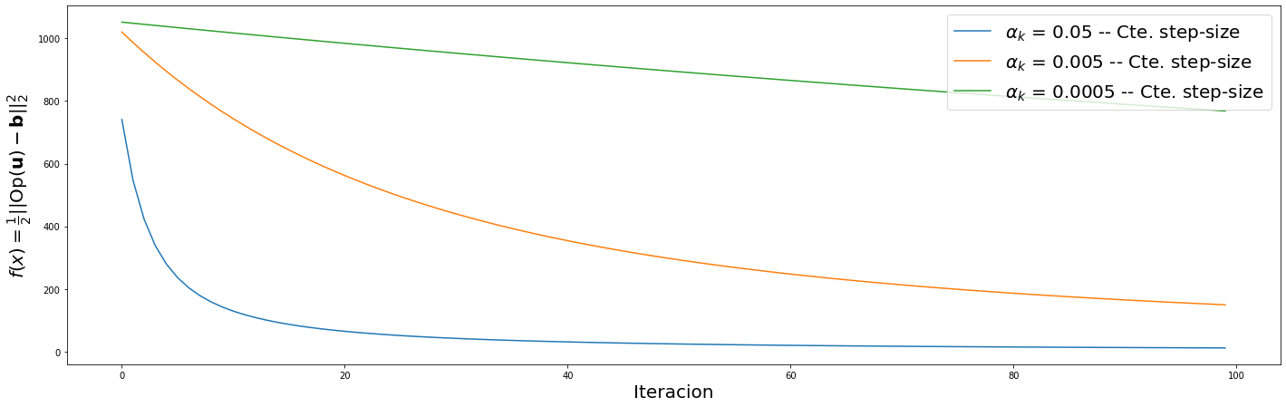
ssCte = [5e-2, 5e-3, 5e-4]
nIter = 100

# Comment the next command out to avoid printing the cost function evolution
args.verbose   = False
args.ssPoliciy = args.f2oDef.ss_Cte

x = []
gdStats = []

for k in range(len(ssCte)):
    args.ssCte     = ssCte[k]
    sol   = gd(Op, b, nIter, args)
    x.append(sol[0])
    gdStats.append(sol[1])

Plot results: cost functional evolution

fig = PLT.figure(figsize=(24, 16))

ax1 = fig.add_subplot(2, 1, 1)

for k in range(len(ssCte)):
    PLT.plot(gdStats[k][:,0], label=r'$\alpha_k$ = {0} -- {1}'.format(ssCte[k], args.f2oDef.ss_list[args.f2oDef.ss_Cte]) )

PLT.legend(loc='upper right',fontsize=20)
PLT.ylabel(r'$f(x) = \frac{1}{2} \|\| $Op$(\mathbf{u}) - \mathbf{b} \|\|_2^2$',fontsize=20)
PLT.xlabel('Iteracion',fontsize=20);